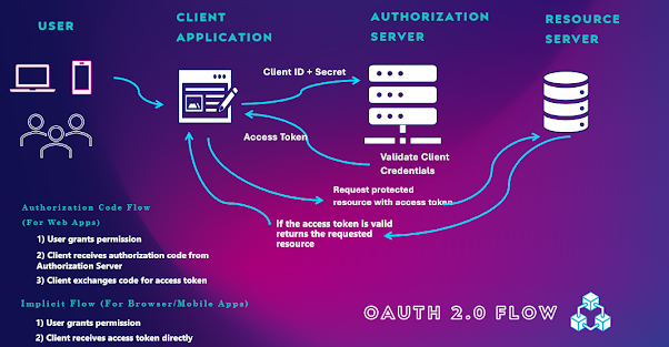
OAuth (Open Authorization) is an open standard for authorization that allow web apps to request access to third party systems on behalf of its users without sharing any account credentials.
OAuth 2.0 is an authorization framework which delegates access and permissions between APIs and applications in a safe and reliable exchange and made more compatible for use by both websites and apps
It also allows for a greater variety of access tokens, like having short-lived tokens and long-lived refresh tokens.
Implement a Data Ingestion Solution Using Amazon Kinesis Video Streams
Create a Kinesis Video Stream for Media Playback
Globomantics is an analytics firm which handles computer vision projects for object detection, image classification, and image segmentation. Your role as a Data Architect is to stream real time video feeds from a source to AWS for further analytics. You'll create a Kinesis Video Stream where live video feeds will later be ingested
Log in to the AWS Console.
Under Find Services, type in and then click Kinesis Video Streams.
Click on Create.
For Video stream name enter VP52M8OQZ10HOQRB, and click on Create video stream.
You will be at the Video streams page for VP52M8OQZ10HOQRB, and in the Video stream info tab the Status will be Active.
Configure Java SDK Producer Library to Stream Video Feeds
In the upper-left click Services, then type in and click on EC2.
Click on Instances (running) and select the instance AnalyticsEngine.
Click on Connect, and at the EC2 Instance Connect tab click Connect. Note: A new browser tab (or window) will open to a Linux command prompt. The EC2 was created for you when you started this lab, and the OS is Ubuntu.
Implement a Data Ingestion Solution Using Amazon Kinesis Data Streams
Create a Kinesis Data Stream
You are a data science consultant for a company called Globomantics, analyzing live temperature feeds. Your primary responsibility is to gather real time data from temperature sensors, and ingest this into a Kinesis Data Stream so that logs can be further analyzed. You will be configuring the Kinesis Data Stream, starting out initially with one shard.
Login to the AWS Console.
Under Find Services, type in and then click Kinesis.
Ensure Kinesis Data Streams is selected, and then click the Create data stream button.
For Data stream name enter RawStreamData.
For Number of open shards enter 1.
Click Create data stream.
Wait for about a minute until the Status of your data stream is Active, at which point it will be ready to accept data streams or a sequence of records.
Connect to an EC2 and Configure Live Temperature Feeds to the Data Stream
Schedule a Python script to send live temperature feeds using the Kinesis API to the data stream you created in the previous challenge.
In the upper-left, click Services, enter EC2 into the search, and click EC2.
In the left panel, under Instances click Instances. Note: You will see an instance named AnalyticsEngine in a Running state, which was created for you when you started this lab.
Select the instance AnalyticsEngine, click Connect, ensure the EC2 Instance Connect tab is selected, then click Connect. Note: A new browser tab will open to a Linux command prompt.
At the command prompt, enter the following two command, replacing and with the CLI CREDENTIALS values provided by this lab.
export AWS_ACCESS_KEY_ID=''
export AWS_SECRET_ACCESS_KEY=''
Note: For example, the first command would look something like
export AWS_ACCESS_KEY_ID='AKIASY3GMJRF5PXADOMT'
Enter cat > sensorstream.py, and paste in this sensorstream.py source code, press enter, then press Ctrl+D. Note: This command creates a script you will next execute, and note there are other ways to do this, such as using vi.
Run the command python sensorstream.py
Note: This ingests live temperature feeds to your Kinesis Data Stream using the python kinesis connector API. If you get an error that ends with something similar to boto.exception.NoAuthHandlerFound: No handler was ready to authenticate. 1 handlers were checked. ['HmacAuthV4Handler'] Check your credentials, then there was an issue with task 4. Double-check things, and re-do that task.
This will start generating temperature feeds, and you will observe continuous sensor data including "iotValue".
Monitor Incoming Data to the Kinesis Data Stream
You generated live temperature feeds and connected them to your Kinesis Data Stream using the Kinesis API. You will monitor the incoming traffic being ingested to the Kinesis Data Stream and based on the increase in load you will increase the number of shards.
Go back to the AWS Console browser tab.
In the upper-left, click Services, enter Kinesis into the search, and click Kinesis.
In the left-hand menu click Data streams, then click the RawStreamData link.
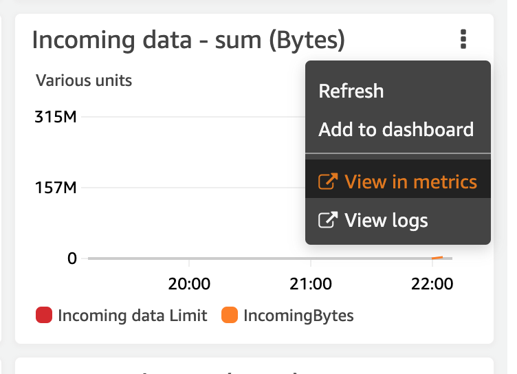
At the RawStreamData page, if needed, click the Monitoring tab. Note: There are various Stream metrics which you can scroll down and see, such as Incoming data - sum (Bytes), Incoming data - sum (Count), Put record - sum (Bytes), Put record latency - average (Milliseconds), and Put record success - average (Percent).
Hover over the Incoming data - sum (Bytes) panel, in its upper-right click the three vertical dots, then click on View in metrics.
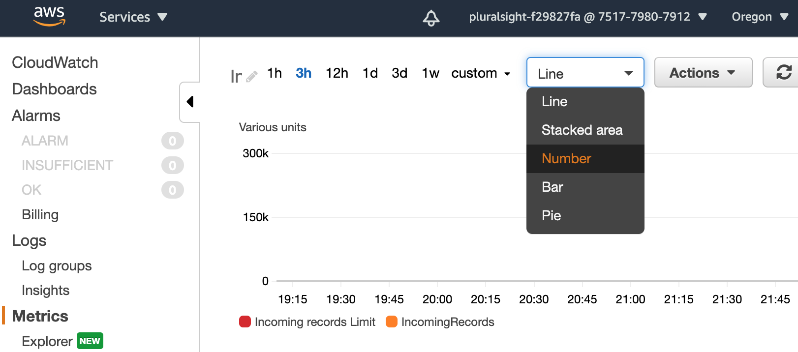
In the new browser tab that opens to the Metric page, select a Number graph. Note: Wait if needed until IncomingRecords is above 1k, which in this scenario will indicate you need more resources to handle the streaming data. The following tasks will show you how to do this by increasing the number of shards.
Go back to the browser tab open to the RawStreamData page, and click the Configuration tab.
Click on Edit, increase the Number of open shards to 2, then click Save changes. Note: This will handle a greater amount of streaming data.
After about a minute, you will see a panel saying Stream capacity was successfully updated for this data stream.
• Create a training and evaluation dataset to be used for batch prediction
• Create a classification (logistic regression) model in BQML
• Evaluate the performance of your machine learning model
• Predict and rank the probability that a visitor will make a purchase
A Subset of visitors who bought on their very first session and then came back and bought again.What are some of the reasons a typical ecommerce customer will browse but not buy until a later visit?
Although there is no one right answer, one popular reason is comparison shopping between different ecommerce sites before ultimately making a purchase decision. This is very common for luxury goods where significant up-front research and comparison is required by the customer before deciding (think car purchases) but also true to a lesser extent for the merchandise on this site (t-shirts, accessories, etc). In the world of online marketing, identifying and marketing to these future customers based on the characteristics of their first visit will increase conversion rates and reduce the outflow to competitor sites.
Create a Machine Learning model in BigQuery to predict whether or not a new user is likely to purchase in the future. Identifying these high-value users can help your marketing team target them with special promotions and ad campaigns to ensure a conversion while they comparison shop between visits to your ecommerce site.
The team decides to test whether these two fields are good inputs for your classification model:
totals.bounces (whether the visitor left the website immediately) totals.timeOnSite (how long the visitor was on our website)
Machine learning is only as good as the training data that is fed into it. If there isn't enough information for the model to determine and learn the relationship between your input features and your label (in this case, whether the visitor bought in the future) then you will not have an accurate model. While training a model on just these two fields is a start, you will see if they're good enough to produce an accurate model.
The inputs are bounces and time_on_site. The label is will_buy_on_return_visit. bounces and time_on_site are known after a visitor's first session. will_buy_on_return_visit is not known after the first visit. Again, you're predicting for a subset of users who returned to your website and purchased. Since you don't know the future at prediction time, you cannot say with certainty whether a new visitor come back and purchase. The value of building a ML model is to get the probability of future purchase based on the data gleaned about their first session. It's often too early to tell before training and evaluating the model, but at first glance out of the top 10 time_on_site, only 1 customer returned to buy, which isn't very promising. Let's see how well the model does.
Create a BigQuery dataset to store models
Select a BQML model type and specify options
Since you are bucketing visitors into "will buy in future" or "won't buy in future", use logistic_reg in a classification model.
You cannot feed all of your available data to the model during training since you need to save some unseen data points for model evaluation and testing. To accomplish this, add a WHERE clause condition is being used to filter and train on only the first 9 months of session data in your 12 month dataset.
After your model is trained, evaluate the performance of the model against new unseen evaluation data.
Evaluate classification model performance
Select your performance criteria:
For classification problems in ML, you want to minimize the False Positive Rate (predict that the user will return and purchase and they don't) and maximize the True Positive Rate (predict that the user will return and purchase and they do).
This relationship is visualized with a ROC (Receiver Operating Characteristic) curve like the one shown here, where you try to maximize the area under the curve or AUC:
In BQML, roc_auc is simply a queryable field when evaluating your trained ML model.
Now that training is complete, you can evaluate how well the model performs with this query using ML.EVALUATE:
You should see the following result:
Row roc_auc model_quality
1 0.724588 decent
After evaluating your model you get a roc_auc of 0.72, which shows the model has decent, but not great, predictive power. Since the goal is to get the area under the curve as close to 1.0 as possible, there is room for improvement.
Improve model performance with Feature Engineering
There are many more features in the dataset that may help the model better understand the relationship between a visitor's first session and the likelihood that they will purchase on a subsequent visit.
Add some new features and create a second machine learning model called classification_model_2:
• How far the visitor got in the checkout process on their first visit
• Where the visitor came from (traffic source: organic search, referring site etc..)
• Device category (mobile, tablet, desktop)
• Geographic information (country)
A key new feature that was added to the training dataset query is the maximum checkout progress each visitor reached in their session, which is recorded in the field hits.eCommerceAction.action_type.
Evaluate this new model to see if there is better predictive power:
Row roc_auc model_quality
1 0.910382 good
With this new model you now get a roc_auc of 0.91 which is significantly better than the first model.
Now that you have a trained model, time to make some predictions.
Predict which new visitors will come back and purchase
Refer the query to predict which new visitors will come back and make a purchase.
The prediction query uses the improved classification model to predict the probability that a first-time visitor to the Google Merchandise Store will make a purchase in a later visit:
The predictions are made on the last 1 month (out of 12 months) of the dataset.
Your model will now output the predictions it has for those July 2017 ecommerce sessions. You can see three newly added fields:
• predicted_will_buy_on_return_visit: whether the model thinks the visitor will buy later (1 = yes)
• predicted_will_buy_on_return_visit_probs.label: the binary classifier for yes / no
• predicted_will_buy_on_return_visit.prob: the confidence the model has in it's prediction (1 = 100%)
Results
• Of the top 6% of first-time visitors (sorted in decreasing order of predicted probability), more than 6% make a purchase in a later visit.
• These users represent nearly 50% of all first-time visitors who make a purchase in a later visit.
• Overall, only 0.7% of first-time visitors make a purchase in a later visit.
• Targeting the top 6% of first-time increases marketing ROI by 9x vs targeting them all!
Additional information
roc_auc is just one of the performance metrics available during model evaluation. Also available are accuracy, precision, and recall. Knowing which performance metric to rely on is highly dependent on what your overall objective or goal is.
AutoML Vision provides an interface for all the steps in training an image classification model and generating predictions on it. Open the navigation menu and and select APIs & Services > Library. In the search bar type in "Cloud AutoML API". Click on the Cloud AutoML API result and then click ENABLE.
Create environment variables for your Project ID and Username:
export PROJECT_ID=$DEVSHELL_PROJECT_ID
export USERNAME=<USERNAME>
Create a Storage Bucket for the images you will use in testing.
Open a new browser tab and navigate to the AutoML UI.
Upload training images to Google Cloud Storage
In order to train a model to classify images of clouds, you need to provide labeled training data so the model can develop an understanding of the image features associated with different types of clouds. Our model will learn to classify three different types of clouds: cirrus, cumulus, and cumulonimbus. To use AutoML Vision we need to put the training images in Google Cloud Storage.
In the GCP console, open the Navigation menu and select Storage > Browser
Create an environment variable with the name of your bucket
export BUCKET=YOUR_BUCKET_NAME
The training images are publicly available in a Cloud Storage bucket. Use the gsutil command line utility for Cloud Storage to copy the training images into your bucket:
Now that your training data is in Cloud Storage, you need a way for AutoML Vision to access it. You'll create a CSV file where each row contains a URL to a training image and the associated label for that image.
Run the following command to copy the file to your Cloud Shell instance:
gsutil cp gs://automl-codelab-metadata/data.csv .
Then update the CSV with the files in your project:
sed -i -e "s/placeholder/${BUCKET}/g" ./data.csv
Navigate back to the AutoML Vision Datasets page.
At the top of the console, click + NEW DATASET.
Type clouds for the Dataset name.
Leave Single-label Classification checked.
Click CREATE DATASET to continue
choose the location of your training images (the ones you uploaded in the previous step)
Choose Select a CSV file on Cloud Storage and add the file name to the URL for the file you just uploaded - gs://your-project-name-vcm/data.csv. You may also use the browse function to find the csv file. Once you see the white in green checkbox you may select CONTINUE to proceed.
After you are returned to the IMPORT tab, navigate to the IMAGES tab. It will take 8 to 12 minutes while the image metadata is processed. Once complete, the images will appear by category.
Inspect images
To see a summary of how many images you have for each label, click on LABEL STATS. You should see the following pop-out box show up on the right side of your browser. Press DONE after reviewing the list.
Train your model
Start training your model! AutoML Vision handles this for you automatically, without requiring you to write any of the model code.
To train your clouds model, go to the TRAIN tab and click START TRAINING.
Enter a name for your model, or use the default auto-generated name.
Leave Cloud hosted selected and click CONTINUE.
For the next step, type the value "8" into the Set your budget box and check "Deploy model to 1 node after training." This process (auto-deploy) will make your model immediately available for predictions after testing is complete.
Click START TRAINING.
The total training time includes node training time as well as infrastructure set up and tear down.
Evaluate your model
After training is complete, click on the EVALUATE tab. Here you'll see information about Precision and Recall of the model. It should resemble the following:
You can also adjust the Confidence threshold slider to see its impact.
Finally, scroll down to take a look at the Confusion matrix.
This tab provides some common machine learning metrics to evaluate your model accuracy and see where you can improve your training data. Since the focus was not on accuracy, move on to the next section about predictions section.
Generate predictions
There are a few ways to generate predictions. Here you'll use the UI to upload images. You'll see how your model does classifying these two images (the first is a cirrus cloud, the second is a cumulonimbus).
First, download these images to your local machine by right-clicking on each of them (Note: You may want to assign a simple name like 'Image1' and 'Image2' to assist with uploading later):
Navigate to the TEST & USE tab in the AutoML UI:
On this page you will see that the model you just trained and deployed is listed in the "Model" pick list.
Click UPLOAD IMAGES and upload the cloud sample images you just saved to your local disk (you may select both images at the same time).
When the prediction request completes you should see something like the following:
The model classified each type of cloud correctly!